Neural Networks: Training The Multi-Layer Perceptron

Training Method

A multi-layer perceptron is trained by presenting it with an input pattern for which the correct response is known and then observing the output. The difference bet­ween correct and observed outputs is the network's overall output error. The neural connection weights within the network are then adjusted to compensate for this measured error.

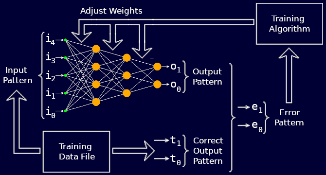
This is repeated for a large number of known examples derived from historic infor­mation about the kind of problem the network is to solve.

Output Error Vector

The input and output patterns are each made up of a set of scalar values. Each scalar value can be imagined as an electrical voltage on one of the pins of an input or output connector. Each scalar value is independent of the others. This independ­ence may be represented pictorially by drawing them at right-angles to each other in vector-space:

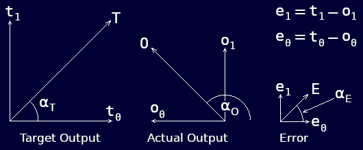
The error vector E above is the difference between the target (or correct) output vector T and the actual output O when a particular input pattern is presented to the network.

[To show the 5-channel input pattern pictorially we would have to draw a graph in 5-dimensional vector space which is rather hard to visualise.]

As can be seen from the above diagram, a vector has both a magnitude and a dir­ection. The direction is denoted by the angle α in each case. In training the network our quest is simply to minimise the magnitude E of the error vector E: its direction is immaterial.

The magnitude E of this vector is given by Pythagoras' Theorem:

In general, for J outputs, the magnitude E of an error vector E is given by the sum­mation below where E is a vector in J-dimensional vector-space:

Output Error Function

To correct large output errors quickly, while gradually easing small errors gently to­wards zero, we can define an error function which is proportional to the square of the actual error. The error function F thus rises ever more rapidly as the errors in the individual output signals increase:

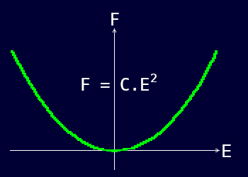
Furthermore, we know that F will always have a positive magnitude. It will therefore be easier to find the point at which it is closest to zero.

Conveniently, the general formula above gives the magnitude of the error vector already squared. Therefore, substituting for E we get:

Our task is to minimise F for every input pattern in the training data file.

Weight Adjustment

While a given fixed input pattern P is being presented to the network, the output (and consequently the error function) can be varied by varying one or more of the weights of the inter-neural links:

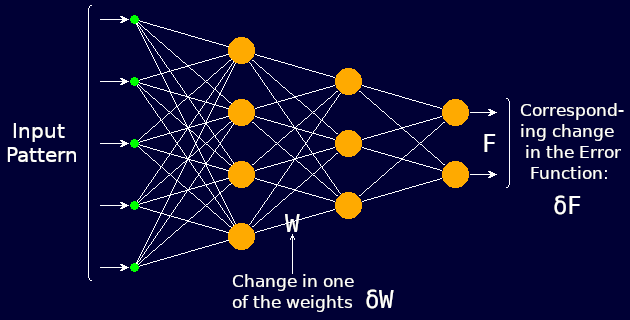
For a fixed input pattern, a change in any one of the weights produces a change in the output pattern. Since the target output pattern is also fixed, a change in any one of the weights produces a corresponding change in the error function F. We can regard F therefore as a function of all the weights in the network, ie.

F = f(w₀,w₁,w₂...w_n)

where 'n' is the number of weights in the network. Holding all the others constant we can therefore plot how varying one of the weights, w causes the error function F to vary:

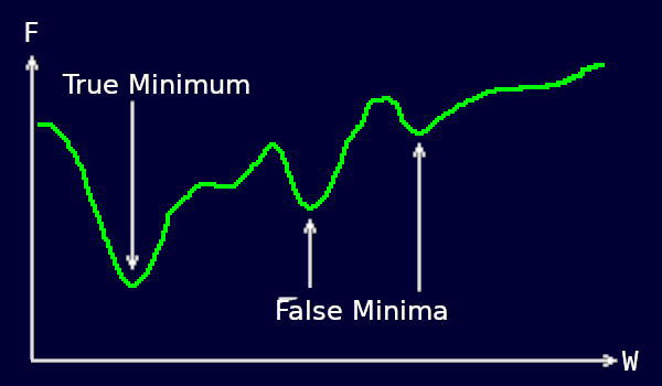
For the current values of all other weights, there should be a value for this weight for which F is a minimum. There could however be other false minima as illustrated above. When adjusting the weights we must try not to get trapped in one of these false minima.

What we need to know is the direction in which we must we adjust a given weight in order to reduce F. Must we increase it or decrease it?

Direction of Adjustment

To find out we must determine which way the curve is sloping at the point on the curve corresponding to the current value of w:

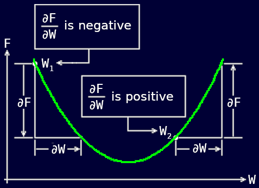
You can see above that for a weight value of w₁ we must increase w to reduce F, and that for a weight value of w₂ we must decrease w to reduce F. Each time we adjust one of the network's weights we must therefore 'add' to it an amount δw which is opposite in sign to the slope of the curve at the point corresponding to the current value of that weight. But by how much? How big do we make δw?

Size of Adjustment

Because F is the square of E we know it will always be positive. We also know that generally, anything squared accelerates in its rate of increase as it gets larger, for example:

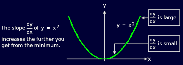
If we make the size of δw proportional to the slope of the curve of F vs w at the point corresponding to the current value of w this will make δw large when F is far from a minimum and small when it is near to a minimum. So w is corrected rapidly when the error is large and slowly when the error is small. With luck this will make the correction process leap over any false minima and settle precisely on the true minimum. But it can't guarantee it.

To adjust each of the network's weights so as to reduce F for a presented input pattern from the training data we must do what in effect is done by the following 'C' statement:

w += delta_w;    //add the weight-increment to the weight

The problem now is to find a viable method of computing ∂F/∂w for any weight w in the network.

Computing ∂F/∂w

To do this we must start with what we know and work back to what we don't know. For each presented input pattern P we know what the output T should be: this is provided in the training data file. We can measure O, the observed output. From these we can compute directly the magnitude of the error function F using the formula:

where J is the number of output channels (which is the same as the number of neurons in the output layer).

Output Error

The contribution to the value of the error function F of a small error δo on 'output pin' j (ie the change in the error function F per unit change in the signal on one of the network's scalar outputs) will therefore be:

After differentiation, the terms of the summation are zero for all except one value of j. The above is therefore the slope of the curve of F vs one output value o_j on a particular output pin j with all the other outputs held constant. To make the maths as simple as possible, we take a little mathematical licence and make C = 1/2 so the above equation becomes:

From the training data file, we know what the output signal t should be on a given output pin j for a given sample input pattern. We can observe the corresponding signal o which the network actually puts out.

The equation above therefore provides us with a measure of how an error in one of the network's output signals (an error in the output from a neuron in the output layer) contributes to the network's output error function F.

Activation Error

Having found how the output 'o' from a single output neuron contributes to the net­work error pattern, we now take a step back to see how this translates into an error in the neuron's activation level 'a'. This is simply how the error in 'o' propagates backwards through the neuron's sigmoid function:

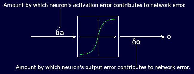
The way an error δa in the activation level 'a' contributes to the network error is therefore given by:

Sigmoid Function

So we now need to find the first derivative do/da of the sigmoid function. Below the sigmoid function is shown with the variables a and o replaced by the more familiar variable names x and y:

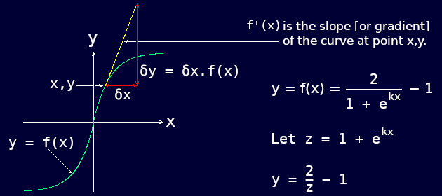
Add corresponding small increments δy and δz to y and z:

Substitute the previous formula for y to get an expression for δy alone:

The first derivative is in effect the slope of the graph of the function at any given point which is dy/dz. Dividing both sides of the above formula by δz:

As δy and δz are made smaller and smaller while preserving their ratio, the terms which are multiplied by δz become insignificantly small compared with those that are not. Therefore the above formula becomes:

Now there is a thing called a chaining rule, which we will not go into here, which states that differential operators behave exactly like algebraic variables in the sense that:

The whole point of the natural number 'e' is that the function 'e' raised to the power 'x' always has the same value as its derivative, ie:

So by the chaining rule:

Since we have already computed 'y' itself, it is convenient to express the derivative in terms of 'y' rather than in 'x' which is more complicated.

Therefore:

Run the program sigdash.exe to generate and display the graph of y = f'(x).
[Source in sigdash.c.]

Finally, substituting our 'neural' variable names, we get the sigmoid's first deriva­tive:

So the change in the network error F resulting from a unit change in the activation level of any neuron is:

Summation Function

We now take a second step further back through the network to see how an error δw, in one of a neuron's input weights 'w', translates into an error δa in the neur­on's activation level 'a'.

To help us to visualise this, we represent the weight 'w' by an electrical rheostat which attenuates the input signal 'i'. An error δw in this weight is therefore repres­ented by a small error in the setting of this rheostat.

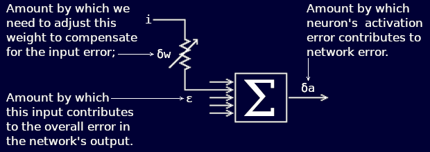
The input signal to the neuron under consideration from a neuron 'i' in the previous layer is i × w. Therefore the error ε in this input signal must be i × δw. The consequ­ential error δa in the neuron's activation level caused by δw must therefore be ε ÷ NI, where NI is the number of inputs to this neuron.

Putting these together:

We now have all the information we need to determine how an error δw in a neur­on's input weight affects the total network error function F.

By the chaining rule:

Substituting for ∂F/∂a and ∂a/∂w:

However, we can only know directly the value of 'o' and ∂F/∂o for neurons in the output layer:

Finding 'o' and ∂F/∂o for neurons in a hidden layer is more complicated.

∂F/∂o for Hidden Neurons

The error in the output of a hidden neuron affects all the network's output signals via its links to the neurons in the next layer. We need therefore to consider the error in the output of a neuron in a hidden layer.

Consider Neuron 0 in the hidden layer just before the output layer. We will refer to this layer as Layer 'j' and the output layer as Layer 'k' as shown below:

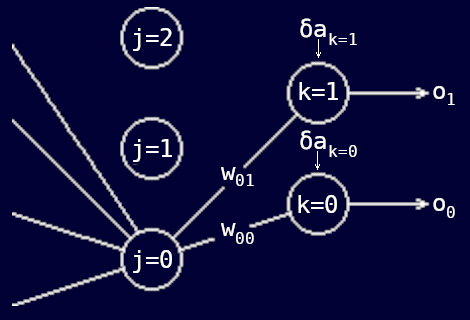
The change δa in the activation level of Neuron k=0 caused by a change in the out­put δo of Neuron j=0 is δo times the weight 'w' on the connecting link between them. Since we will be implementing our network using 16-bit interger arithmetic we must divide this by NI, the number of inputs to the neurons in Layer 'k', ie:

The error in the activation level of Neuron k=0 per unit error in the output of Neur­on j=0 is therefore:

In general, therefore, for any link between Layer 'j' and Layer 'k' the above expres­sion becomes:

What we are looking for is the contribution to the value of the network output error function F produced by the error in the output of Neuron j=0, namely:

By the chaining rule:

because the errors in both the links contribute to the error in the network's output. In general, therefore, for a network with an output layer containing K neurons:

∂F/∂a for Hidden Neurons

Next we have to find how this error in a hidden neuron's output translates into an error in its activation level. Using the chaining rule and substituting for ∂F/∂a and ∂a/∂w (as we did previously for an output neuron) we get:

Note: the index k is a different variable from the k in the second brace.

Hidden Neuron's Inputs

We must now back-track further to consider the weights on the inputs to Neuron j=0:

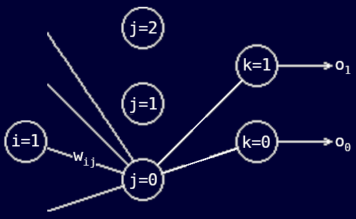
We must find how the error δw in the weight 'w' (see above) on one of Neuron j=0's input links affects the neuron's output. The internal function of hidden neurons is exactly the same as that of the neurons in the output layer. The formula for finding how an error in one of its input weights affects its output is therefore the same, namely:

∂F/∂w for Hidden Neurons

We now have all the information we need to determine how an error δw in a hidden neuron's input weight affects the total network error function F. So by the chaining rule:

Rationalisation

We need two separate expressions for computing ∂F/∂w:
for output neurons:

and for hidden neurons:

Adjusting Output Weights

When a pattern is presented to the network, the network function mlp() computes and stores the outputs of all the neurons in the network starting with the first hid­den layer and progressing through to the output layer. We therefore know 'o' and 'i' for every neuron in the network.

In the case of output layer neurons therefore we have all we need directly to com­pute ∂F/∂w for each input weight of each neuron and 'add' to it the appropriate amount:

So before considering any of the hidden layers we will go ahead and adjust the input weights to the output layer.

Adjusting Hidden Weights

We also know 'o' and 'i' for hidden neurons and, having just adjusted the input weights to the output layer, we know these also.

But notice that the summation term in the 'hidden' formula needs the value of ∂F/∂a for each neuron in Layer 'k', the output layer (assuming for the moment that we are considering the hidden layer immediately before the output layer). We must there­fore save the output layer's values of ∂F/∂a while we have them; i.e. while we are adjusting the output layer's weights. Then we can pick them up when we come to process the hidden layer.

BACK-PROPAGATION

This process of computing and expediting the weight adjustments for the output layer and then using this for computing and expediting the weight adjustments for the hidden layer behind it is called back-propagation.

Similarly, while computing and expediting the weight adjustments for the hidden layer immediately behind the output layer, we save its values of ∂F/∂a namely:

for when we come to compute and expedite the weight adjustments for the hidden layer immediately behind that one. And so on until we get to the first hidden layer in the network namely the one next to the input.

Training Algorithm

The training algorithm for adjusting the weights in response to the error F, which results when a given training pattern P is processed by the mlp() function, is shown in a kind of pseudo 'C' below:

For each layer of the network 
(working backwards from the output):
{
  for each neuron in the layer
  {
    compute ∂F/∂a;
    store it for use next pass of the loop;

    for each input weight to the neuron
    {
      compute ∂F/∂w;
      w −= h * ∂F/∂w;      //adjust the weight
    }
  }
}

In practice, faster code can be produced by splitting the computation of ∂F/∂a between successive passes of the loop. Full implementation in 'C' of this training algorithm is covered in this document.

Data Structure

The mlp training algorithm uses the same data structure as the mlp( ) 'C' function described in mlp.html. However, we need to add extra arrays to hold the output errors for each layer. We also need an extra array T[] to hold the correct outputs corresponding to each set of presented inputs. The original data structure with these extra arrays added is shown below:

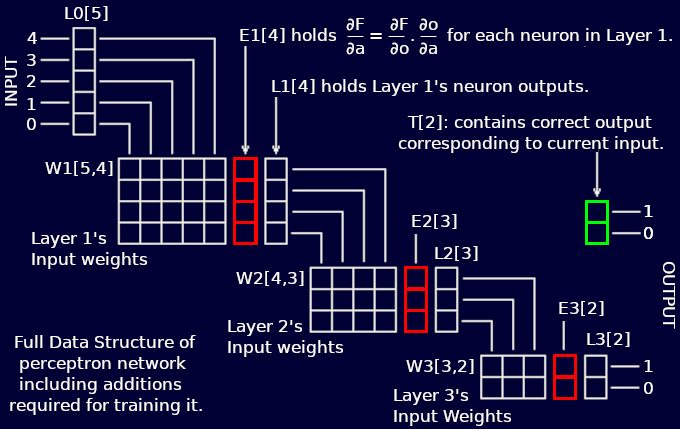
As in mlp( ), we need to re-organise this data structure to take advantage of the 'C' language's pointer arithmetic capabilities. An extra pointer array L[] is required to access the output arrays for the different layers. Another extra pointer array E[] is similarly required to access the error array for the different layers:

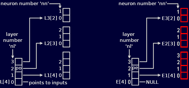
Pointer variable po = *(L + nl) is used in conjunction with a neuron number 'nn' within the layer 'nl' in order to access the output 'o' of a given neuron. So the output of a given neuron, o = *(po + nn). The corresponding pointer variable pe = *(E + nl) is used similarly to access a neuron's activation level error. So the activation error for a given neuron, ∂F/∂a = *(pe + nn).

The method of accessing the inter-neural connection weights is the same exactly as it was in the mlp( ) function discussed in document mlp.html. It is repeated below for convenience:

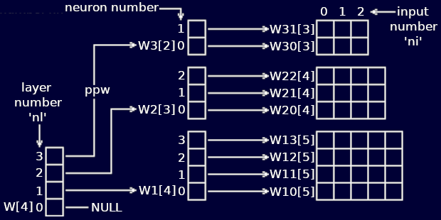
Note that one more order of indirection is needed for weights. A 'pointer to a pointer' variable ppw = *(W + nl) is established which is used to set up the pointer variable pw = *(ppw + nn). A given weight is then obtained using pw so that w = *(pw + ni).

Training Procedure

The training procedure is a matter of adjusting the weights of the network until the observed output is as close a match as possible to the correct output provided in the training data file. Finding out by how much and in which direction each weight must be altered and then doing the alteration must be done as a number of sepa­rate computational steps as follows:

Step 1:

Each element of the output layer's error array must be primed with the relative amount by which each neuron's output signal affects the overall output function F as follows:

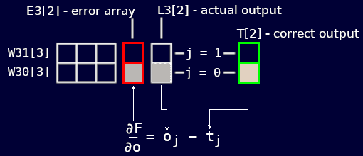
The index 'j' signifies the neuron number 'nn' of a neuron within the output layer. This corresponds to the element number of each of the three arrays where the correct output, observed output and error differential relating to that neuron are stored. A program loop must be used to work out the error differential ∂F/∂o for each value of j, ie for each neuron in the output layer.

Step 2:

The error differential of each neuron's output signal must then be replaced by the error differential of its activation level. In other words we want to find how the error differential is propagated back through the neuron's sigmoid function. We saw earl­ier that this is given by:

To do this we lift ∂F/∂o out of the appropriate element of the error array E3[], multiply it by ∂o/∂a for which we get 'o' from the corresponding element of the output array L3[] and place the result back in the same element of the error array as illustrated below:

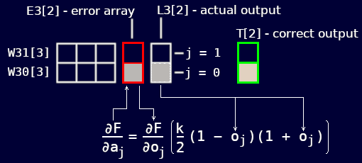
Again a program loop must be used to work out the error differential ∂F/∂a for each value of 'j', i.e. for each neuron in the output layer.

Step 3:

Now we can adjust the output layer's input weights. The inputs to this layer are the outputs from the previous layer. We therefore signify them by the letter 'o' subscr­ipt­ed by the index 'i' indicating the neuron number 'nn' within the previous layer ['j' indicates the neuron number 'nn' within this layer]. The weight adjustment process is illustrated below:

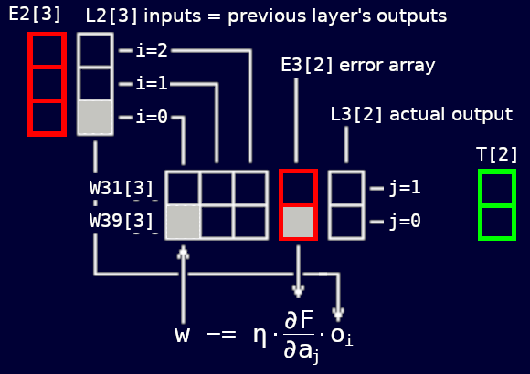
The weights are adjusted in the following way. The weight on each input to the first neuron (j = 0) is adjusted in turn. We start with the weight on input i = 0 and finish with the weight on input i = 2.

In general, if there are I neurons in the previous layer, we start with the weight on input i = 0 and finish by adjusting the weight on input i = I − 1.

We then do the same for the weights on the inputs to the second neuron (j = 1). In general, if there are J neurons in the layer we are dealing with then we do the same for the weights on the inputs to the other neurons.

To do all this we need two nested program loops:

for(j = 0; j < J; j++)
  for(i = 0; i < I; i++)
    W[i][j] −= eta * E3[j] * L2[i];

Please note that unlike Java and other modern programming languages, C code does not support non-ASCII letters such as Greek letters. So for η we must substitute its name in English: 'eta'. However, provided the text editor supports the full UTF-8 character set, you can put Greek letters etc. in the program comments [/* ... */] of a C-program.

Direct reference to array elements by the indexes i and j has been used above rather than pointer references. This is to help you understand the process more clearly at this stage.

Step 4:

Finally we must prime the previous layer's error array with ∂F/∂o ready for when we come to process that layer in the next program pass.

We prime the error array at this stage because the items we need are easier to reference from the point of view of the current layer than from the point of view of the previous layer. [Note that because we are working backwards through the net­work the previous layer is the next layer to be processed.]

The process of calculating ∂F/∂o for the first neuron of the previous layer is illustr­ated below:

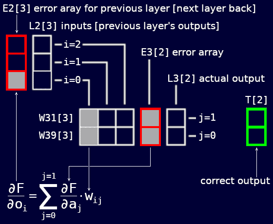
The value of ∂F/∂o is got by adding up the products of each pair of horizontally corresponding weight and error elements, i.e. you add the product of E3[0] and W30[0] to the product of E3[1] and W31[0].

The weight elements required to obtain the values of ∂F/∂o for the second and third elements of E2[] are shown below:

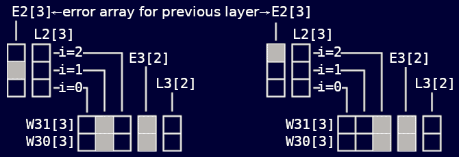
Having primed the error array for the previous layer we loop back to Step 2 and re­peat Steps 2 though 4 with the array indexing set to the point of view of the prev­ious layer. We then loop through Steps 2 through 3 a third time to perform them with respect to the second layer back from the output layer.

Kolmogorov's Theorem implies [as I was given to understand at the time of writing] that a three-layer perceptron can handle any func­tion. Consequently we never need more than three active layers. Therefore on this third and final pass of the loop we do not need to do Step 4 since there are no fur­ther error arrays to prime.

The Training Function

Skeleton 'C' Function

These 4 steps have been put together within an appropriate layer control loop to form the skeleton 'C' function below:

               /* pointer to inputs       
                     |          pointer to true outputs
                     |          |       shift factor to multiply by η / R
                     |          |       |  */
void mlptrain(short *pi, short *pt, int h) {
  for(nl = NAL; nl > 0; nl−−) { //for each layer of the network
    if(nl == NAL) { //If doing output layer (i.e. first time thru) 
      PRIME EACH ELEMENT OF THE ERROR ARRAY WITH −(t[j] − o[j]).
    }
    for(nn = 0; nn < NN; nn++) { //for each neuron in this layer
      MULTIPLY NEURON'S PRIMED ERROR VALUE BY ∂o/∂a
      THEN ADJUST ALL THIS NEURON'S INPUT WEIGHTS
    }
    if(nl > 1) {   //If not yet reached first active layer 
      PRIME THE PREVIOUS LAYER'S ERROR ARRAY ELEMENTS
      WITH THIS LAYER'S ERROR * WEIGHT SUMMATIONS.
    }
  }
}

This expands into a complete 'C' function as follows:

The Complete 'C' Function

short
  E1[N1], E2[N2], E3[N3],     // output errors for each layer
  *E[] = {NULL, E1, E2, E3};  // array of ptrs to above arrays

                  /* pointer to inputs       
                     |          pointer to true outputs
                     |          |       shift factor to multiply by η / R
                     |          |       |  */
void mlptrain(short *pi, short *pt, int h) {
  int nl;     // layer number
  L[0] = pi;  // points to start of network inputs array
  h += 15;    // shift factor to multiply by η / R

  for(nl = NAL; nl > 0; nl−−) {  //for each layer of the network
    short 
      **ppw = *(W + nl),   // ptr to access layer's weights
      *pe = *(E + nl),     // ptr to layer's output errors
      *po = *(L + nl);     // ptr to layer's neural outputs
    int 
      nn, NN = *(N + nl),  // neuron number within current layer
      NI = *(N − 1 + nl);  // number of inputs to this layer
    if(nl == NAL)          // If doing output layer, 

      // Prime each element of the error array with −(t[j] − o[j])
      for(nn = 0; nn < NN; nn++)
        *(pe + nn) = *(po + nn) − *(pt + nn);

    pi = *(L + nl − 1);  // ptr to start of layer's inputs

    // For each neuron in this layer, compute the output error
    for(nn = 0; nn < NN; nn++) {
      short *pw = *(ppw + nn);  // ptr to neuron's first weight 
      long o = *(po + nn),      // this neuron's output signal
           e = (((R + o) * (R − o)) >> 15) * *(pe + nn)) >> 13;
      if(e >  R) e =  R; 
      if(e < −R) e = −R;
      *(pe + nn) = e;  // ∂F/∂a = ∂o/∂a * last time's summation
      for(ni = 0; ni < NI; ni++)  // adjust each input weight
        *(pw + ni) −= ((e * *(pi + ni)) / NI) >> h;
    }
    if(nl > 1) {                    // If not yet reached 1st active layer
      short *ps = *(E + nl − 1);    // ptr to prev layer's output errors
      for(ni = 0; ni < NI; ni++) {  // for each input weight to this layer
        long Hi = 0, Lo = 0;        // see mlp() to explain following code
        for(nn = 0; nn < NN; nn++) {
          long P = (long)*(pe + nn) * *(*(ppw + nn) + ni);
          Hi += P >> 16; Lo += P & 0xFFFF;
        }
        *(ps + ni) = ((Hi << 1) + (Lo >> 15)) / NN;
      }
    }   // End prime previous layer's error array elements 
  }     // with this layer's error * weight summations.
}

Overview

A training example comprises one input pattern plus its corresponding correct out­put pattern. The training data file contains a number of training examples which to­gether represent the full range of patterns to which the network is being trained to respond.

The function mlptrain() adjusts the network's weights to minimise the error bet­ween the network's output and the known correct output for each given training example. The function is therefore called once after each training example has been present­ed to the network.

[A training example is presented to the network by calling the function mlp() discussed in the document MLP.html.]

The function mlptrain() is therefore called once for each example in the training data file. The constant of proportionality η is then reduced and the process re­peated. This is done until the error function F for each training example cannot be reduced any further.

Please refer to the complete 'C' function listing while reading the following.

Input Arguments

The function mlptrain() has to be told where to find its inputs by means of a pointer pi which is passed to it as an input argument. Immediately after entry this value is placed in pointer array element L[0]. The pointer pi is then used in the rest of the function to point to the input values pertaining to the neuron currently being pro­ces­sed.

However, mlptrain( ) also needs to be told where to find the correct output respons­es corresponding to those inputs. We let it know this by means of a second pointer pt which we pass to it as a second input argument.

The constant of proportionality η must be reduced externally to mpltrain() for suc­cessive presentations of the training data file. It must therefore be passed to the mlptrain() function as an argument.

In the 'C' code, instead of multiplying the weight increment by η, we right-shift it by an amount 'h'. For example if η = ¼ then h = 2. Since we are using interger arithmetic, we add 15 to this right-shift factor to give it the effect of dividing by R (the maximum interger value).

The prototyped envelope of mlptrain( ) must therefore be:

void mlptrain(short *pi, short *pt, int h) { }

Declarations

The neural input, output and weights arrays are declared externally within the mlp source file. Only the additional error arrays E1[], E2[] and E3[] plus their associated pointer array E[] need to be declared for mlptrain(). The start addresses of E1[], E2[] and E3[] are placed in the elements of E[]. E[0] is primed with a NULL pointer value because there is no error array E0[] for the input layer since the input layer has no active neurons.

Layer Loop

The outermost loop in mlptrain() steps from the output layer backwards through the network finishing with the active layer next to the input layer. Thus the passive input layer is Layer 0, the first active layer is Layer 1 and the output layer is Layer 3. The constant NAL (Number of Active Layers) is defined externally within the mlp source file. Its value is in fact 3. The layer loop thus comprises the statements:

int nl;
for (nl = NAL; nl > 0; nl−−) {
}

The layer number nl starts equal to 3 and the loop is executed for nl = 3. The vari­able nl is then decremented (by nl−−) and the loop is executed for nl = 2. It is then decremented again and the loop is executed for nl = 1. It is then decremented again whereupon it becomes zero and therefore the test nl > 0 fails so the loop terminates without executing for nl = 0.

Pointers

The first task done inside the layer loop is to set up pointers to point to the input weights, the output values and output errors for the layer concerned. The pointer variable ppw is a pointer-to-a-pointer-to-an-interger. It is set equal to the address found in the nl^th element of the pointer array W[] by the statement:

ppw = *(W + nl);

It points to the start address of one of the secondary pointer arrays W3[], W2[] or W1[] according to the current value of nl. Since ppw is not referred to outside the Layer Loop, the statement in the actual function also declares it as a pointer to a pointer to a short interger at the same time viz:

short **ppw = *(W + nl),

The pointer pe is set up to point to the start address of the layer's error array E3[], E2[] or E1[] according to the current value of nl. Since it too is not referred to out­side the layer loop, the setting up statement also declares it:

*pe = *(E + nl),

Since the declaration for ppw was terminated by a comma instead of a semi-colon, the word 'short' does not have to be repeated.

Finally, the pointer variable po is set to point to the start address of the layer's out­put array L3[], L2[] or L1[] according to the current value of nl:

po = *(L + nl);

This is declared in the same way as the other two, and for the same reason as be­fore, the 'short' type word does not have to be repeated.

Neuron Loop

We now need to deal with each neuron in turn within the current layer nl. To do this we establish a loop within the layer loop which we shall call the Neuron Loop. For this we need an interger variable nn (neuron number) to tell us which of this layer's neurons we are currently dealing with. We therefore declare nn:

int nn;

We also need to know how many neurons there are in this layer. This is held in the appropriate element of the array N[]. This array is declared globally and initialised in the mlp source file. The number of neurons NN in Layer Nº nl is therefore N[nl]. We therefore declare and assign NN as:

int NN = *(N + nl);

We therefore establish the neuron loop within the layer loop as follows:

int nn, NN = *(N + nl);
for(nn = 0; nn < NN; nn++) {
}

Note that unlike the layers we can count the neurons upwards from 0 to NN − 1. In fact we need to loop through all the neurons in the current layer up to 3 times, each time doing something quite different.

Priming The Output Errors

If we are on the very first pass of the Layer Loop (ie we are dealing with the output layer) we first need to prime the error array E3[] with −(t_nn − o_nn) for each neuron.

The pointer pe points to the start address of this layer's error array, E3[], i.e. it points to the error array element corresponding to this layer's Neuron Nº 0.

The pointer value pe + nn therefore points to the element of this layer's error array which contains the error value corresponding to this layer's Neuron Nº nn. In gen­eral, i.e. for any layer nl, the situation is as follows:

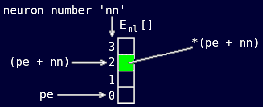
The error value epsilon_nn is therefore the contents of the array element whose address is pe + nn. The error value ε_nn for Neuron Nº nn is therefore given by ε_nn = *(pe + nn).

In the same way, the values for the given correct output for a given neuron nn and the observed output for the neuron nn are given by:

t_nn = *(pt + nn) and o_nn = *(po + nn)

The error differential ∂F/∂o for each output neuron is therefore computed by the statement:

*(pe + nn) = *(po + nn) − *(pt + nn);

The complete program fragment for priming the error array for the output layer is therefore:

if(nl == NAL)                   //If doing output layer, 
  //Prime each element of the error array with  −(t[j] − o[j])
  for(nn = 0; nn < NN; nn++)
    *(pe + nn) = *(po + nn) − *(pt + nn);

Syntactically the above is a single 'C' statement so no braces are needed.

Activation Error

Having primed each of the output layer's error array elements with ∂F/∂o for each output neuron we now have to multiply each by do/da (the first differential of the Sigmoid function) and replace it with the resulting activation error differential ∂F/∂a.

We first have to get the neuron's output value 'o'. Because we are about to multiply integers we will obtain 'o' as a 'long' 32-bit interger as follows so that we do not lose any precision from the 32-bit product:

long o = *(po + nn);

This ensures that even though other operands in the multiplication may be only 16-bit integers, the product will have full 32-bit precision.

We can then compute ∂F/∂a (which we shall call 'e') as follows:

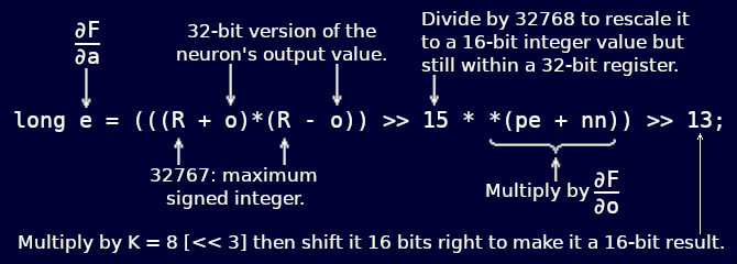
The terms (R + o) and (R − o) are scaled to a maximum absolute value of 32768. Their product is therefore scaled to the square of 32768. To bring the scale of the product back to 32768 we divide it by 32768. We achieve this by right-shifting it 15 places (32768 is the 15^th power of 2).

Be aware that although it has been right-shifted 15 binary places to scale it back to 32768, the product (R + o) * (R − o) is still held as a 32-bit 'long' quantity. This ensures that before it is multiplied by ∂F/∂o, ∂F/∂o is itself converted to a 'long' so that the full 32-bit precision of the resulting 'long' product is preserved.

Finally, we shift this 'long' (32-bit) product into a 'short' (16- bit) register by right-shifting the whole lot 16 places.

However at this point we also need to multiply the result by the sigmoid's shaping constant k. Since it has been decided to make k = 8 we simply need to left-shift our result by 3. So that we hold on to as many of the least-significant bits in the final result as possible, we combine the right-shift of 16 and the left-shift of 3 as a single right-shift of 13.

The resulting value of ∂F/∂a is then stored into the neuron's output error array element.

The complete program fragment for converting ∂F/∂o to ∂F/∂a for each neuron in this layer is therefore:

// For each neuron in this layer, compute the output error.
for(nn = 0; nn < NN; nn++) {
  long
    o = *(po + nn),  // this neuron's output signal
    e = (((R + o) * (R − o)) >> 15) * *(pe + nn)) >> 13; 
  if(e >  R) e =  R;
  if(e < −R) e = −R;
  *(pe + nn) = e;    // ∂F/∂a = ∂o/∂a * ∂F/∂o
}

The activation error differential ∂F/∂a is stored as a 'short' interger. Since in the final scaling we are shifting only 13 binary places right instead of 16 there is a remote possibility that the result could overflow 16-bits. That is the reason for the range-limiting 'if' statements above just before the result is stored.

Weight Adjustments

Two levels of indirection are required to access weights. As well as ppw we there­fore need a second pointer pw which points directly to the start address of the weights on the inputs to a neuron nn in layer nl. How these two pointers relate and how an individual weight value is addressed is illustrated below:

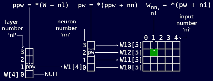
Since the value of ppw is constant for a given layer, we have already set it up at the start of the layer loop. But here we need to set up pw which we declare and as­sign at the same time as follows:

short *pw = *(ppw + nn);   //pointer to neuron's first weight

To adjust the input weights to a neuron we need to know the strengths of its input signals from the previous layer. These of course are the output signals generated by the neurons in the previous layer. These are held in the previous layer's output array L_(nl−1) []. So if we are adjusting Layer 3's weights we will find each neuron's input signals in L2[].

To address a neuron's inputs we therefore need to set up another pointer to point to the start address of the previous layer's outputs array L_(nl−1)[] as follows:

pi = *(L + nl − 1);   //pointer to start of this layer's inputs

For this purpose we have made use of the now-redundant input argument pointer variable pi.

Each input weight of the neuron we are currently dealing with must be adjusted by an amount:

Using the pointers we have just set up to address the operands we can now im­plement this within mlptrain() as follows:

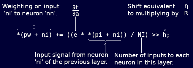
Since 'e' is a 'long', the product e * *(pi + ni) is evaluated as a 'long'. Both 'e' and *(pi + ni) are scaled to an absolute maximum of R (= 32768). Their product is there­fore scaled to R-squared. To re-scale the right-hand side to 32768 we need to divide by R. That is why 'h', the shift factor equivalent of η was increased by 15 at the beginning of mlptrain().

The activation level error differential ∂F/∂a is contributed to by the errors in all the inputs to the neuron concerned. We therefore divide by the number of inputs to the neuron, NI. To preserve as much precision as possible we do this division before doing the right-shift.

The complete program fragment for adjusting the input weights of one neuron (Neuron Nº nn of Layer Nº nl) is as follows:

short *pw = *(ppw + nn);  //pointer to neuron's first weight 
pi = *(L +nl − 1);        //ptr to start of this layer's inputs
//Adjust the input weight for each input to this neuron
for(ni = 0; ni < NI; ni++)
  *(pw + ni) −= ((e * *(pi + ni)) / NI) >> h;

Since this must be done for all the neurons in the current layer, the above program fragment must go inside the neuron loop immediately following the computation of ∂F/∂a.

The updating of the current layer is now finished.

Priming the Next Layer

Because we have the pointers pe and ppw already set up, it is more convenient to prime the previous layer's error array with the required values for ∂F/∂o now rather than at the start of the next pass of the layer loop. All we lack is a way to address the elements of the previous layer's error array E_(nl−1)[]. We provide this by declar­ing and assigning a pointer ps to point to the start address of E_(nl−1)[] as follows:

//pointer to previous layer's output errors
short *ps = *(E + nl − 1);

Remember that we can only get ∂F/∂o directly in the case of the output layer, and we have already done it for the output layer. Whichever pass of the layer loop we are on, the previous layer at this point is necessarily always a hidden layer. We must therefore compute its ∂F/∂o values using the summation formula:

To maintain full precision for the product of the activation error differential ∂F/∂o and the weight wni,nn we cast one of them to a 'long' and assign the result to a 'long' variable:

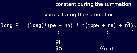
Notice that since we are stepping between the weights arrays during the summa­tion loop we cannot simply assign pw = *(ppw + nn) since nn is a variable during the loop. Looking at the weight matrix, we are stepping vertically up the matrix instead of across it as we were in previous loop.

We need to accumulate the sum of these 'long' products without losing precision or risking overflow. We achieved this by the split accumulator method shown below:

long Hi = 0, Lo = 0;
for(nn = 0; nn < NN; nn++) {
  long P = (long)*(pe + nn) * *(*(ppw + nn) + ni);
  Hi += P >> 16;
  Lo += P & 0xFFFF;
}

The 'long' product P is split into upper and lower 'short' halves. Each half is added into a separate Hi and Lo 'long' accumulator. This is repeated for nn = 0 to NN − 1. At the end of the summation loop the upper half of the Lo accumulator is added to the Hi accumulator to form a 'long' summation as follows:

*(ps + ni) = ((Hi << 1) + (Lo >> 15)) / NN;

The summation is then divided by the number of neurons in the current layer in order to rescale the sum to a 'short'. The result is the value of ∂F/∂o for this neuron which is then stored in the appropriate element ni of E_(nl−1)[].

The split accumulator summation is used in the 'neuron' part of the mlp() function which is described in the document neuron.html and is fully exercised and demon­strated by the program neuron.c.

This summation must be done for every neuron in the previous layer (i.e. the next layer back towards the network's input). We must therefore set the summation loop within another loop which steps through each neuron of that previous layer:

//pointer to previous layer's output errors
short *ps = *(E + nl − 1);
for (ni = 0; ni < NI; ni++) {  //for each input to this layer
  DO THE SUMMATION LOOP
  *(ps + ni) = ((Hi << 1) + (Lo >> 15)) / NN;
}

Since the neurons of the previous layer provide the inputs for the current layer, the previous layer's error array E_(nl−1)[] has NI elements. Consequently, we can use the same loop arrangement we used earlier to adjust the input weights. To address the elements of the previous layer's error array we can therefore use the input index ni in conjunction with a new pointer ps which we must declare outside the loop where we must also set it to point to the start address of the previous layer's error array E_(nl−1)[].

The last error array we need to prime is E1[], the first hidden layer of the network (ie the first active layer following the passive input layer). There are no connection weights on the direct inputs to the network from the outside world. Therefore there is no array called E0[]. We prime E1[] during the pass of the layer loop in which we are dealing with Layer 2. Therefore we must only perform this priming process for Layers 3 and 2. We must therefore condition the execution of the error array prim­ing with an 'if' statement as follows:

if(nl > 1) {  //If not yet reached 1st active layer 
  PRIME THE PREVIOUS LAYER'S ERROR ARRAY
}

We have now reached the end of the layer loop. We therefore, at this point, loop back to do the previous layer (the next layer back towards the input) until we have dealt with all the layers of the network.

Rearrangements

Notice that in the listing of the complete 'C' function I have relocated some of the pointer declaration/assignment statements so that they are no longer immediately next to the program fragments to which they each directly relate. This is simply to avoid them being repeatedly set up within a loop in which they are constants.

Adding Momentum

The training of a multi-layer perceptron cannot be guaranteed. Training is not a completely deterministic process. This is because during training, the network can become settled on to false minima of the error function.

There is an enhancement we can make to the training algorithm which can help reduce the risk of the network becoming trapped in a false minimum. This is by ad­ding what we call a momentum term to the weight adjustment.

You will recall that the amount by which each weight in the network should be ad­justed is given by:

When homing in on a minimum (whether the true one or a false one) the size of δw is getting smaller and smaller. What we want to do is introduce a degree of slug­gishness into the rate at which δw becomes smaller. We do this by adding in last time's value of δw as follows:

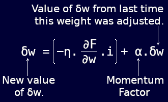
The value of δw will thus exhibit a characteristic analogous to momentum which tends to resist our efforts to reduce it. The hope is that this will tend to bull­doze the weight clean over small localised minima where the weight is being adjust­ed rapid­ly (i.e. where δw is large), while allowing the weight to settle gently on to the true minimum where the weight is being adjusted slowly (i.e. where δw is small).

In our 'C' programming notation we could write the full process of adjusting a weight 'w' as:

However, as well as storing the adjusted weight 'w' as before, we must also save the weight increment δw so that it is available the next time we adjust this weight. We must therefore declare a set of arrays M which is a replica of that for the weights arrays.

This new array structure with the new pointer variables ppm and pm for accessing them are as shown below:

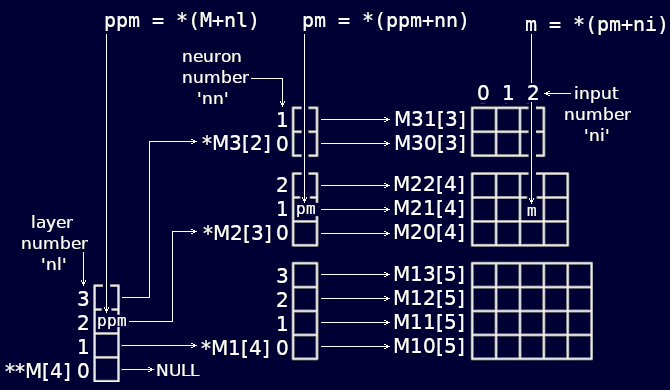
To implement the 'momentum term' enhancement we must declare these new ar­rays within the 'C' source file as follows:

M10[N0],M11[N0],M12[N0],M13[N0],  // Layer 1 input delta-weights
M20[N1],M21[N1],M22[N1],          // Layer 2 input delta-weights
M30[N1],M31[N1],                  // Layer 3 input delta-weights
*M1[] = {M10, M11, M12, M13},     // Access to L1 delta-weights
*M2[] = {M20, M21, M22},          // Access to L2 delta-weights
*M3[] = {M30, M31},               // Access to L3 delta-weights
**M[] = {NULL, M1, M2, M3},       // Access to all delta-weights

Next, at the start of the appropriate loop in the mlptrain() function, we must de­clare the additional pointers we need to access the new array structure:

short **ppm = *(W + nl);  // ptr to access layer's delta-weights
short *pm = *(ppm + nn);  // ptr to neuron's first delta-weight

Finally we must expand the weight adjustment statement itself:

The Enhanced 'C' Function

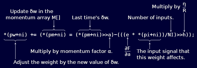
The complete 'C' function mlptrain() is reproduced below with the added code for the momentum term enhancement statements shown in bold.

The new M[] arrays have been declared inside the function since they are not refer­red to from outside mlptrain() as things stand. However, if it is likely that training runs will exceed a day, it may be expedient to shut off the computer at night. In this case the current states of all arrays will have to be saved to disk and re-loaded in the morning. For this to be possible, all arrays will have to be defined externally so that the disk I/O function can access them as well.

                  /* pointer to input pattern array
                     |          pointer to 'correct' output pattern array
                     |          |       Shift factor corresponding
                     |          |       |  to weight gain term η.
                     |          |       |      Shift factor corresponding 
                     |          |       |      |  to Momentum Factor α.
                     |          |       |      |  */
void mlptrain(short *pi, short *pt, int h, int a) {
  short
    E1[N1],E2[N2],E3[N2],    // output errors for each layer
    *E[] = {NULL,E1,E2,E3},  // array of ptrs to above arrays

    M10[N0],M11[N0],M12[N0],M13[N0], // Layer 1 input δw
    M20[N1],M21[N1],M22[N1],         // Layer 2 input δw
    M30[N1],M31[N1],                 // Layer 3 input δw
    *M1[] = {M10, M11, M12, M13},    // Access to L1 δw
    *M2[] = {M20, M21, M22},         // Access to L2 δw
    *M3[] = {M30, M31},              // Access to L3 δw
    **M[] = {NULL, M1, M2, M3};      // Access to all δw

  int nl;       // layer number
    L[0] = pi;  // points to start of network inputs array
    h += 15;    // shift factor to multiply by η / R

  for(nl = NAL; nl > 0; nl−−) {  // for each layer of network
    short 
      **ppw = *(W + nl),   // ptr to this layer's weights
      **ppm = *(W + nl),   // ptr to layer's delta-weights
      *pe = *(E + nl),     // ptr to layer's output errors
      *po = *(L + nl);     // ptr to this layer's outputs
    int 
      nn, ni,              // neuron number, input number
      NN = *(N + nl),      // number of neurons in layer
      NI = *(N − 1 + nl);  // number of inputs to layer

    /* If processing the output layer, prime each element 
       of the error array with −(t[j] − o[j]). */
    if(nl == NAL)
      for (nn = 0; nn < NN; nn++)
        *(pe + nn) = *(po + nn) − *(pt + nn);

    pi = *(L + nl − 1);  // pointer to start of layer's inputs

    //Compute the output error for each neuron in this layer.
    for(nn = 0; nn < NN; nn++) {
      short 
        *pw = *(ppw + nn),  // ptr to neuron's first weight 
        *pm = *(ppm + nn);  // ptr to neuron's 1st delta-weight
      long 
        o = *(po + nn),     // this neuron's output signal
        e = (((R + o) * (R − o)) >> 15) * *(pe + nn) >> 13; 

      if(e > R) e = R; if(e < −R) e = −R;
      *(pe + nn) = e;  // ∂F/∂a = ∂o/∂a * last time's summation

      for(ni = 0; ni < NI; ni++)  // adjust each input weight
        *(pw + ni) += (
                        *(pm +ni) = (*(pm + ni) >> a) 
                                  − (((e * *(pi + ni)) / NI) >> h)
                      );
    }
    if(nl > 1) {                    // if not yet reached 1st active layer 
      short *ps = *(E + nl − 1);    // ptr to prev layer's output errors
      for(ni = 0; ni < NI; ni++) {  // for each input weight to this layer
        long Hi = 0, Lo = 0;        // see mlp() to explan the following code
        for(nn = 0; nn < NN; nn++) {
          long P = (long)*(pe + nn) * *(*(ppw + nn) + ni);
          Hi += P >> 16; Lo += P & 0xFFFF;
        }
        *(ps + ni) = ((Hi << 1) + (Lo >> 15)) / NN;
      }
    }   // ... prime the previous layer's error array elements 
  }     //     with this layer's error * weight summations. 
}

This code is stored in the file train.c. It is useful to study it in a highlighting text editor such as gedit. I mostly prefer gedit's Cobalt theme's highlighting for viewing code, although sometines I like to revert to the default Classic theme.

Overflow Considerations

The sizes of the operands in the enhanced weight adjustment statement are shown below:

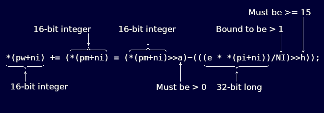
Provided a > 0 (ie we are dividing last time's δw by at least 2) then the momen­tum term can never exceed ±R/2. Provided h is at least 15, the delta term can never exceed ±R/2. So the difference between them (no matter what their signs) can never exceed ±R. The updated value of δw can never therefore exceed ±R. [R = 32767.]

---

© December 1997 Robert John Morton